Dynamic Time Warping¶

Dynamic Time Warping (DTW) 1 is a similarity measure between time series. Let us consider two time series \(x = (x_0, \dots, x_{n-1})\) and \(y = (y_0, \dots, y_{m-1})\) of respective lengths \(n\) and \(m\). Here, all elements \(x_i\) and \(y_j\) are assumed to lie in the same \(d\)-dimensional space. In tslearn, such time series would be represented as arrays of respective shapes (n, d) and (m, d) and DTW can be computed using the following code:

from tslearn.metrics import dtw, dtw_path

dtw_score = dtw(x, y)
# Or, if the path is also an important information:
optimal_path, dtw_score = dtw_path(x, y)

Optimization problem¶

DTW between \(x\) and \(y\) is formulated as the following optimization problem:

\[DTW(x, y) = \min_\pi \sqrt{ \sum_{(i, j) \in \pi} d(x_i, y_j)^2 }\]

where \(\pi = [\pi_0, \dots , \pi_K]\) is a path that satisfies the following properties:

it is a list of index pairs \(\pi_k = (i_k, j_k)\) with \(0 \leq i_k < n\) and \(0 \leq j_k < m\)
\(\pi_0 = (0, 0)\) and \(\pi_K = (n - 1, m - 1)\)
for all \(k > 0\) , \(\pi_k = (i_k, j_k)\) is related to \(\pi_{k-1} = (i_{k-1}, j_{k-1})\) as follows:
- \(i_{k-1} \leq i_k \leq i_{k-1} + 1\)
- \(j_{k-1} \leq j_k \leq j_{k-1} + 1\)

Here, a path can be seen as a temporal alignment of time series such that Euclidean distance between aligned (ie. resampled) time series is minimal.

The following image exhibits the DTW path (in white) for a given pair of time series, on top of the cross-similarity matrix that stores \(d(x_i, y_j)\) values.

Code to produce such visualization is available in our Gallery of examples.

Algorithmic solution¶

There exists an \(O(mn)\) algorithm to compute the exact optimum for this problem (pseudo-code is provided for time series indexed from 1 for simplicity):

def dtw(x, y):
    # Initialization
    for i = 1..n
        for j = 1..m
            C[i, j] = inf

    C[0, 0] = 0.

   # Main loop
   for i = 1..n
        for j = 1..m
            dist = d(x_i, y_j) ** 2
            C[i, j] = dist + min(C[i-1, j], C[i, j-1], C[i-1, j-1])

   return sqrt(C[n, m])

Using a different ground metric¶

By default, tslearn uses squared Euclidean distance as the base metric (i.e. \(d(\cdot, \cdot)\) in the optimization problem above is the Euclidean distance). If one wants to use another ground metric, the code would then be:

from tslearn.metrics import dtw_path_from_metric
path, cost = dtw_path_from_metric(x, y, metric=compatible_metric)

in which case the optimization problem that would be solved would be:

\[DTW(x, y) = \min_\pi \sum_{(i, j) \in \pi} \tilde{d}(x_i, y_j)\]

where \(\tilde{d}(\cdot, \cdot)\) is the user-defined ground metric, denoted compatible_metric in the code snippet above.

Properties¶

Dynamic Time Warping holds the following properties:

\(\forall x, y, DTW(x, y) \geq 0\)
\(\forall x, DTW(x, x) = 0\)

However, mathematically speaking, DTW is not a valid distance since it does not satisfy the triangular inequality.

Additional constraints¶

The set of temporal deformations to which DTW is invariant can be reduced by setting additional constraints on the set of acceptable paths. These constraints typically consists in forcing paths to lie close to the diagonal.

First, the Sakoe-Chiba band is parametrized by a radius \(r\) (number of off-diagonal elements to consider, also called warping window size sometimes), as illustrated below:

../_images/sakoe_chiba.png — \(n = m = 10, r = 3\). Diagonal is marked in grey for better readability.¶

The corresponding code would be:

from tslearn.metrics import dtw
cost = dtw(x, y, global_constraint="sakoe_chiba", sakoe_chiba_radius=3)

Second, the Itakura parallelogram sets a maximum slope \(s\) for alignment paths, which leads to a parallelogram-shaped constraint:

../_images/itakura.png — \(n = m = 10, s = 2\). Diagonal is marked in grey for better readability.¶

The corresponding code would be:

from tslearn.metrics import dtw
cost = dtw(x, y, global_constraint="itakura", itakura_max_slope=2.)

Alternatively, one can put an upper bound on the warping path length so as to discard complex paths, as described in 2:

from tslearn.metrics import dtw_limited_warping_length
cost = dtw_limited_warping_length(x, y, max_length)

Barycenters¶

Computing barycenter (also known as Fréchet means) of a set \(\mathcal{D}\) for DTW corresponds to the following optimization problem:

\[\min_\mu \sum_{x \in \mathcal{D}} DTW(\mu, x)^2\]

Optimizing this quantity can be done through the DTW Barycenter Averaging (DBA) algorithm presented in 3.

from tslearn.barycenters import dtw_barycenter_averaging
b = dtw_barycenter_averaging(dataset)

This is the algorithm at stake when invoking tslearn.clustering.TimeSeriesKMeans with metric="dtw".

soft-DTW¶

DTW is not differentiable with respect to its inputs because of the non-differentiability of the min operation. A differentiable extension has been presented in 4 in which the min operator is replaced by soft-min, using the log-sum-exp formulation:

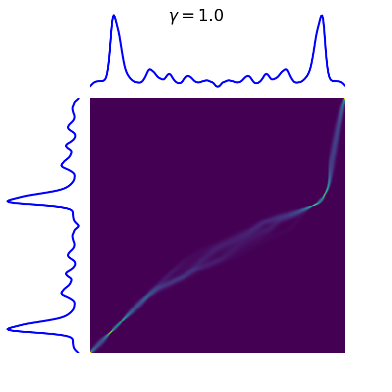
\[\text{soft-min}_\gamma(a_1, \dots, a_n) = - \gamma \log \sum_i e^{-a_i / \gamma}\]

soft-DTW hence depends on a hyper-parameter \(\gamma\) that controls the smoothing of the resulting metric (squared DTW corresponds to the limit case \(\gamma \rightarrow 0\)).

from tslearn.metrics import soft_dtw
soft_dtw_score = soft_dtw(x, y, gamma=.1)

When a strictly positive value is set for \(\gamma\), the corresponding alignment matrix corresponds to a blurred version of the DTW one:

Also, barycenters for soft-DTW can be estimated through gradient descent:

from tslearn.barycenters import softdtw_barycenter
b = softdtw_barycenter(dataset, gamma=.1)

This is the algorithm at stake when invoking tslearn.clustering.TimeSeriesKMeans with metric="softdtw".

Examples Involving DTW variants¶

Longest Common Subsequence

Canonical Time Warping

Dynamic Time Warping

Soft Dynamic Time Warping

DTW computation with a custom distance metric

Barycenters

Soft-DTW weighted barycenters

References¶

1: H. Sakoe, S. Chiba, “Dynamic programming algorithm optimization for spoken word recognition,” IEEE Transactions on Acoustics, Speech and Signal Processing, vol. 26(1), pp. 43–49, 1978.
2: Z. Zhang, R. Tavenard, A. Bailly, X. Tang, P. Tang, T. Corpetti Dynamic time warping under limited warping path length. Information Sciences, vol. 393, pp. 91–107, 2017.
3: F. Petitjean, A. Ketterlin & P. Gancarski. A global averaging method for dynamic time warping, with applications to clustering. Pattern Recognition, Elsevier, 2011, Vol. 44, Num. 3, pp. 678-693
4: M. Cuturi, M. Blondel “Soft-DTW: a Differentiable Loss Function for Time-Series,” ICML 2017.