Longest Common Subsequence
Longest Common Subsequence (LCSS) [1] is a similarity measure between time series.
Let us consider two time series \(x = (x_0, \dots, x_{n-1})\) and
\(y = (y_0, \dots, y_{m-1})\) of respective lengths \(n\) and
\(m\).
Here, all elements \(x_i\) and \(y_j\) are assumed to lie in the same
\(d\)-dimensional space.
In tslearn, such time series would be represented as arrays of respective
shapes (n, d) and (m, d) and LCSS can be computed using the following code:
from tslearn.metrics import lcss, lcss_path

lcss_score = lcss(x, y)
# Or, if the path is also an important information:
path, lcss_score = lcss_path(x, y)
Problem
The similarity \(S\) between \(x\) and \(y\), given a positive real number \(\epsilon\), is formulated as follows:
The constant \(\epsilon\) is the matching threshold.
Here, a path can be seen as the parts of the time series where the Euclidean distance between them does not exceed a given threshold, i.e., they are close/similar.
To retrieve a meaningful similarity value from the length of the longest common subsequence, the percentage of that value regarding the length of the shortest time series is returned.
Algorithmic solution
There exists an \(O(n^2)\) algorithm to compute the solution for this problem (pseudo-code is provided for time series indexed from 1 for simplicity):
def lcss(x, y):
   # Initialization
   for i = 0..n
       C[i, 0] = 0
   for j = 0..m
       C[0, j] = 0

   # Main loop
   for i = 1..n
        for j = 1..m
            if dist(x_i, x_j) <= epsilon:
                C[i, j] = C[i-1, j-1] + 1
            else:
                C[i, j] = max(C[i, j-1], C[i-1, j])

   return C[n, m] / min(n, m)
Using a different ground metric
By default, tslearn uses squared Euclidean distance as the base metric
(i.e. \(dist()\) in the problem above is the
Euclidean distance). If one wants to use another ground metric, the code
would then be:
from tslearn.metrics import lcss_path_from_metric
path, cost = lcss_path_from_metric(x, y, metric=compatible_metric)
Properties
The Longest Common Subsequence holds the following properties:
\(\forall x, y, LCSS(x, y) \in \left[0, 1\right]\)
\(\forall x, y, LCSS(x, y) = LCSS(y, x)\)
\(\forall x, LCSS(x, x) = 1\)
The values returned by LCSS range from 0 to 1, the value 1 being taken when the two time series completely match.
Additional constraints
One can set additional constraints to the set of acceptable paths. These constraints typically consists in forcing paths to lie close to the diagonal.
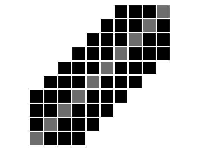
First, the Sakoe-Chiba band is parametrized by a radius \(r\) (number of off-diagonal elements to consider, also called warping window size sometimes), as illustrated below:

\(n = m = 10, r = 3\). Diagonal is marked in grey for better readability.
The corresponding code would be:
from tslearn.metrics import lcss
cost = lcss(x, y, global_constraint="sakoe_chiba", sakoe_chiba_radius=3)
The Sakoe-Chiba radius corresponds to the parameter \(\delta\) mentioned in [1], it controls how far in time we can go in order to match a given point from one time series to a point in another time series.
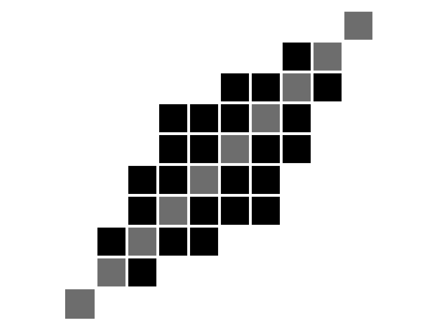
Second, the Itakura parallelogram sets a maximum slope \(s\) for alignment paths, which leads to a parallelogram-shaped constraint:

\(n = m = 10, s = 2\). Diagonal is marked in grey for better readability.
The corresponding code would be:
from tslearn.metrics import lcss
cost = lcss(x, y, global_constraint="itakura", itakura_max_slope=2.)
Examples Involving LCSS variants

Longest Commom Subsequence with a custom distance metric